Both data flow performance and diagnostic metric sources just presented help you determine where to start with your optimization effort. From both a source and sink perspective, recall the configurations available through their numerous tabs, for example, Projection and Optimize, as shown in Figure 5.21, Figure 4.26, and Figure 5.22. Tightening the columns of data you bring from the source onto the platform for transformation can increase performance. Projecting and tightening data means that you remove unnecessary columns from the query that retrieves the data, thus reducing the amount of data. If this is an option, then the Projection tab on the source is the place to perform that. For both the source and sink data, you are provided with an option to set partitioning. In each case, for both the source and sink, the data needs to be physically located in some datastore and in some format. In step 5 of Exercise 5.6, you selected the round‐robin distribution model into which the sink data will be structured onto the node, and you left the default of Use Current Partitioning for the source. The other options for defining the structure of your transformed data are Hash, Dynamic Range, Fixed Range, and Key. As you’ve read in many examples in this book, the distribution model you choose depends on how your data is used.

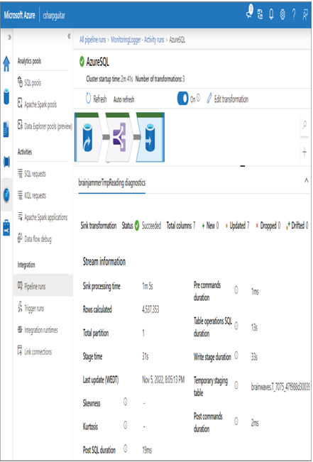
FIGURE 10.10 Optimizing pipelines for analytics or transactional purposes: data flow sink transformation

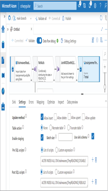
Another option for optimizing a sink is to disable indexes prior to loading the data into the sink. Indexes are a must‐have when retrieving data from a data table; however, indexes slow insert operations. You can disable indexes by executing the following SQL commands:

ALTER INDEX ALL ON brainwaves.[TmpREADING] DISABLE
ALTER INDEX ALL ON brainwaves.[TmpREADING] REBUILD

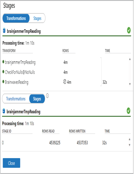
Remember that part of the integration dataset configuration of a sink is to identify the location, which includes the table, into which the data will be written. That table is the one on which you disable and then reapply the indexes during the data flow execution. There are two multiline text boxes on the Settings tab of the data flow, as shown in Figure 10.12, where you can add Pre SQL scripts and Post SQL scripts. You can also see them in Figure 10.11, along with the duration each took.

FIGURE 10.11 Optimizing pipelines for analytics or transactional purposes: data flow transformations

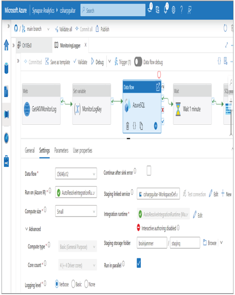
Configuring the pipeline to execute data flows in parallel is another option for improving sink performance. When you have multiple data flows within your pipeline that can run in parallel, then you can implement that by selecting the Run in Parallel check box for the given data flow, as shown in Figure 10.13.

The Compute Size, Compute Type, and Core Count drop‐downs enable you to scale the resources allocated to a data flow. Table 10.7 shows the options in the Compute Size drop‐down.

TABLE 10.7 Data Flow Compute size

Compute size	Compute type	Core count
Small	Basic (General Purpose)	4 (+ 4 Driver cores)
Medium	Basic (General Purpose)	8 (+ 8 Driver cores)
Large	Standard (Memory Optimized)	16 (+ 16 Driver cores)

FIGURE 10.12 Optimizing pipelines for analytics or transactional purposes: data flow pre and post SQL scripts

FIGURE 10.13 Optimizing pipelines for analytics or transactional purposes: data flow parallel execution