Data shuffling was introduced in Chapter 2, where it was described as the movement of data from one node to another. When using the hash distribution model, remember that the distribution key provided to the HASH function determines how the data is organized across the compute nodes. Review Figure 2.10 to visualize this. It is common that datasets partitioned by the distribution key are so large that they must be spread across multiple nodes. Data shuffling is observed when a query is executed that must pull data from more than a single node. In other words, when a query is executed, the SQL statement is run on a single node. If the data required to gather and process that query completely exists on a partition on the same node as the one running the SQL statement, then no data shuffling is required. However, if only a portion of the data is on a partition where the SQL statement is running, then the platform, or the massively parallel processing (MPP) engine, must know where the other required data is hosted and retrieve it. Refer to Figure 2.9 to visualize the MPP engine. The amount of data shuffling depends on the amount of retrieved data, the distribution key, and the complexity of the SQL statement.

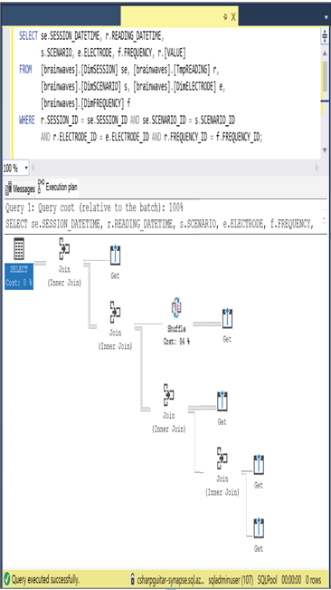
In addition to data shuffling, Chapter 2 introduced the DDL command EXPLAIN. Using the EXPLAIN command results in XML output, which mimics the visualization from Figure 9.23. Both the XML and its illustration are the location where you can find occurrences and details about data shuffling as it pertains to the specific SQL query. Figure 10.5 illustrates how the second JOIN in the SQL query is affected by a shuffle cost of 86 percent. This means that 86 percent of the data necessary to complete that join is located on a node other than the one executing the SQL statement.

The XML file includes additional details, including operation_type=SHUFFLE_MOVE. The cost value, which is rendered in Figure 10.5, is an estimated amount of time required to run the operation; accumulative_cost is the sum of all costs in the plan; average_rowsize is the estimated row size in bytes of retrieved rows during the operation; and output_rows is the number of rows retrieved during the operation. Comparing these values can give you some insights into the impact of data shuffling. Keep in mind that all data shuffling is not bad. When you see it happening, you need to review the impact and then determine if actions are required.

FIGURE 10.5 Finding shuffling in a pipeline—explain plan with shuffle cost

From a Spark pool perspective, there are two methods for identifying data shuffling. The first method is to use the explain method with syntax similar to the following, which you might recognize from Exercise 5.15:

If there are remnants of data shuffling, they would be associated with the keyword Exchange. You can determine the impact by reviewing the associated details. The other method to find data shuffling is to view the directed acyclic graph (DAG), which was introduced in Chapter 9 and illustrated in Figure 9.26. When data shuffling is happening, you will also see an Exchange statement followed by a Shuffle statement.